Predicting NFL Playoffs

Introduction

Professional sports tend to have a lot of inertia. The best teams in one season tend to be contenders the next season as well. Although players get shuffled around through trades, free agency, drafts, and waivers, the full cast of players on each team doesn’t change that much from year to year.

The NFL is a prime example of a high inertia league. The New England Patriots have only missed the playoffs 3 times in the last 17 years whereas the Cleveland Browns last playoff appearance was a Wild Card loss in 2002. To find the last Browns playoff win you have to go all the way back to 1994 (where they beat the Patriots in a Wild Card game). Granted, these teams are on extreme ends of the spectrum. But the point remains that teams tend to mirror performance of the previous year, making gains/losses on the multi-season time scale as opposed to the sub-seasonal (week-to-week) or seasonal time scale.

Recently I stumbled onto this visualization which breaks down offensive positional spending vs in-season success of NFL teams. I saw some interesting things such as the most successful teams (13-16 wins) spent less on wide receivers and quarterbacks and more on running backs and tight ends than teams with 12 wins or less.

This then begged the question: could I use this positional spending data and previous season team performance to predict what teams were going to make the playoffs this year? Only one way to find out…

Getting the Data

The data that I wanted for this project was positional spending, number of players at each position, and offensive/defensive stats from the previous year. I also needed to grab NFL standings for each year which includes features like wins, losses, point differential, made playoffs, etc. This served as my target variable in some way, I’ll get to that later.

Unfortunately, this data was not readily available in a tidy csv. Also, since there’s a single table for each team, season, and feature, I couldn’t simply copy and paste the tables into Excel and create a csv that way. I needed to scrape the data systematically from several websites and then consolidate the data into a single dataset. To do this I used Python’s Requests and BeautifulSoup packages. Positional spending came from Spotrac.com, offensive/defensive data came from NFL.com, and season standings data came from ESPN.com.

The code for scraping the data is in notebooks 1.1 - 1.4 here.

Positional spending data was only available for the 2013-2018 seasons so that is the time scope of this project. Previous year stats were taken from 2012-2017, where one year was added to match with the current year’s positional salary.

After scraping the data, each set was saved into separate csv files. Merging the csv files together yielded a dataset of 39 independent variables and 192 observations (32 teams * 6 years) as well as a set of potential dependent variables.

Feature Descriptions

Below is a description of each of the independent features that was scraped from the websites mentioned above.

Team - Team abbreviation (2 or 3 characters)

Year - Year of start of season

Team Stats (Previous Year)

TO - Turnover differential

Offensive Stats (Previous Year)

Yds/G_rush_off - Yards per game rushing by offense
TD_rush_off - Number of rushing touchdowns by offense
Yds/G_pass_off - Yards per game passing by offense
Pct_off - Completion percentage by offense
TD_pass_off - Number of passing touchdowns by offense
Sck_off - Number of sacks allowed by offense
Rate_off - Quarterback rating by offense
Pts/G_off - Points per game by the offense
Pen Yds_off - Penalty yards by offense

Defensive Stats (Previous Year)

Yds/G_rush_def - Yards per game rushing allowed by defense
TD_rush_def - Number of rushing touchdowns allowed by defense
Yds/G_pass_def - Yards per game passing allowed by defense
TD_pass_def - Number of passing touchdowns allowed by defense
Rate_def - Quarterback rating allowed by defense
Sck_def - Number of sacks by defense
Pct_def - Completion percentage allowed by defense
Pts/G_def - Points per game allowed by defense
Pen Yds_def - Penalty yards by defense

Salary Spending by Position (Current Year)

QB - Quarterback salary
RB - Running back salary
WR - Wide receiver salary
TE - Tight end salary
OL - Offensive line salary
DL - Defensive line salary
LB - Linebacker salary
S - Secondary salary
ST - Special teams salary

Number of Players per Position (Current Year)

nQB - Number of quarterbacks
nRB - Number of running backs
nWR - Number of wide receivers
nTE - Number of tight ends
nOL - Number of offensive linemen
nDL - Number of defensive linemen
nLB - Number of linebackers
nS - Number of secondary players
nST - Number of special teams players

Potential Target Variables

W - Number of wins
L - Number of losses
T - Ties
PF - Points for
PA - Points against
DIFF - Point differential (PF-PA)
Playoffs - Made playoffs (1 = made playoffs, 0 = didn’t make playoffs)
SB_win - Won Superbowl (1 = won superbowl, 0 = didn’t win superbowl)

Exploratory Data Analysis

I always look at the correlation matrix first to get a feel for how each variable is related.

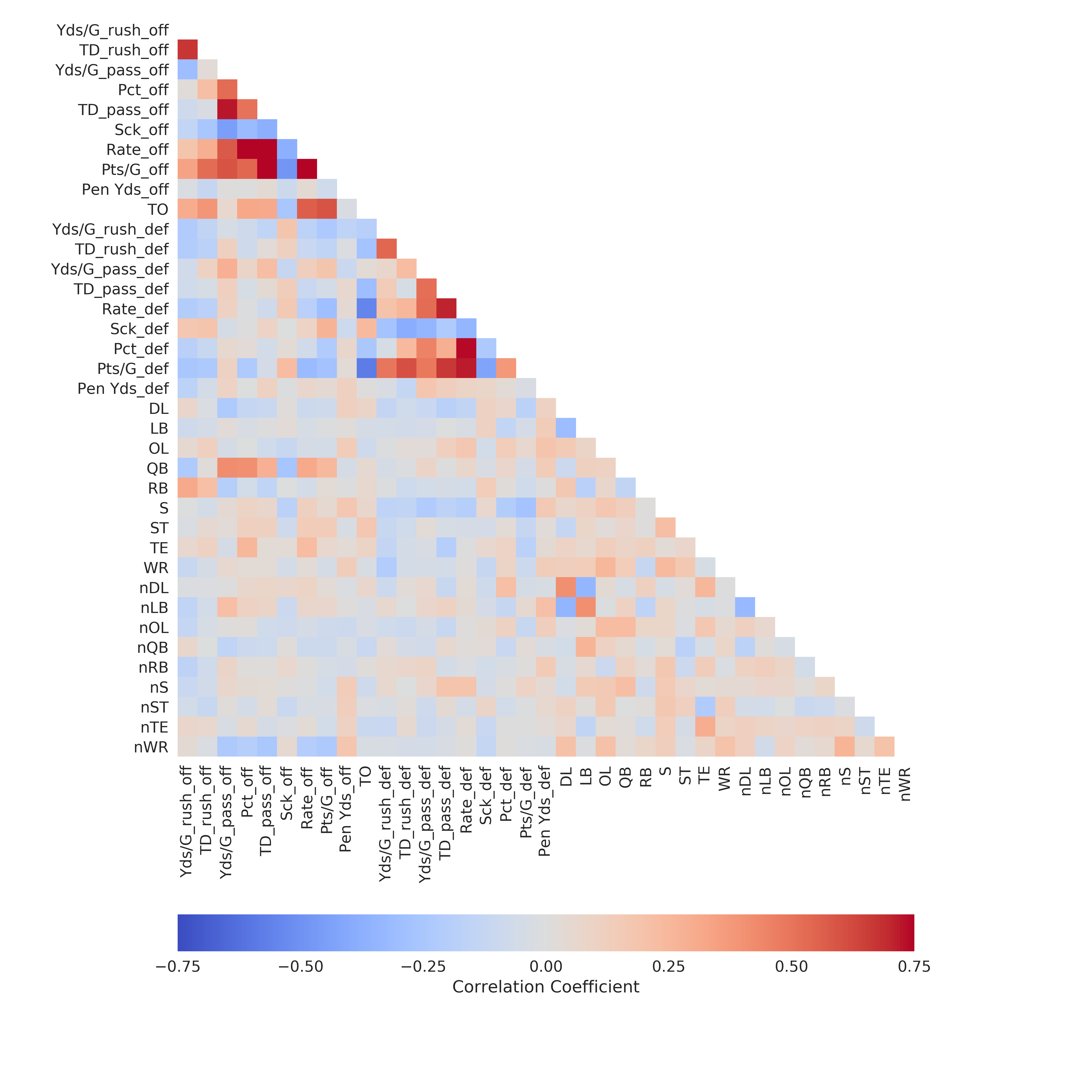
It’s not surprising that the offensive features are highly correlated. For instance, the correlation between passer rating and completion percentage is 0.81. Below is the formula used by the NFL to calculate passer rating.

The first term in the numerator $\frac{COMP}{ATT}$ is, in fact, completion percentage. There are other factors involved in calculating the passer rating which is why the correlation between passer rating and completion percentage is not 1.0.

If I was using straight linear regression on all of the independent features, I would need to remove variables which are highly correlated with each other. I’ll actually be using some feature selection techniques later so I don’t need to bother with that at this point.

Next, I’ll look at the correlation between each independent variable and the number of wins to see which variables have the strongest individual relationship with my target variable. Keep in mind that the team statistics are from the prior season and the positional salary and number of positional players are from the same season as when the wins were recorded.

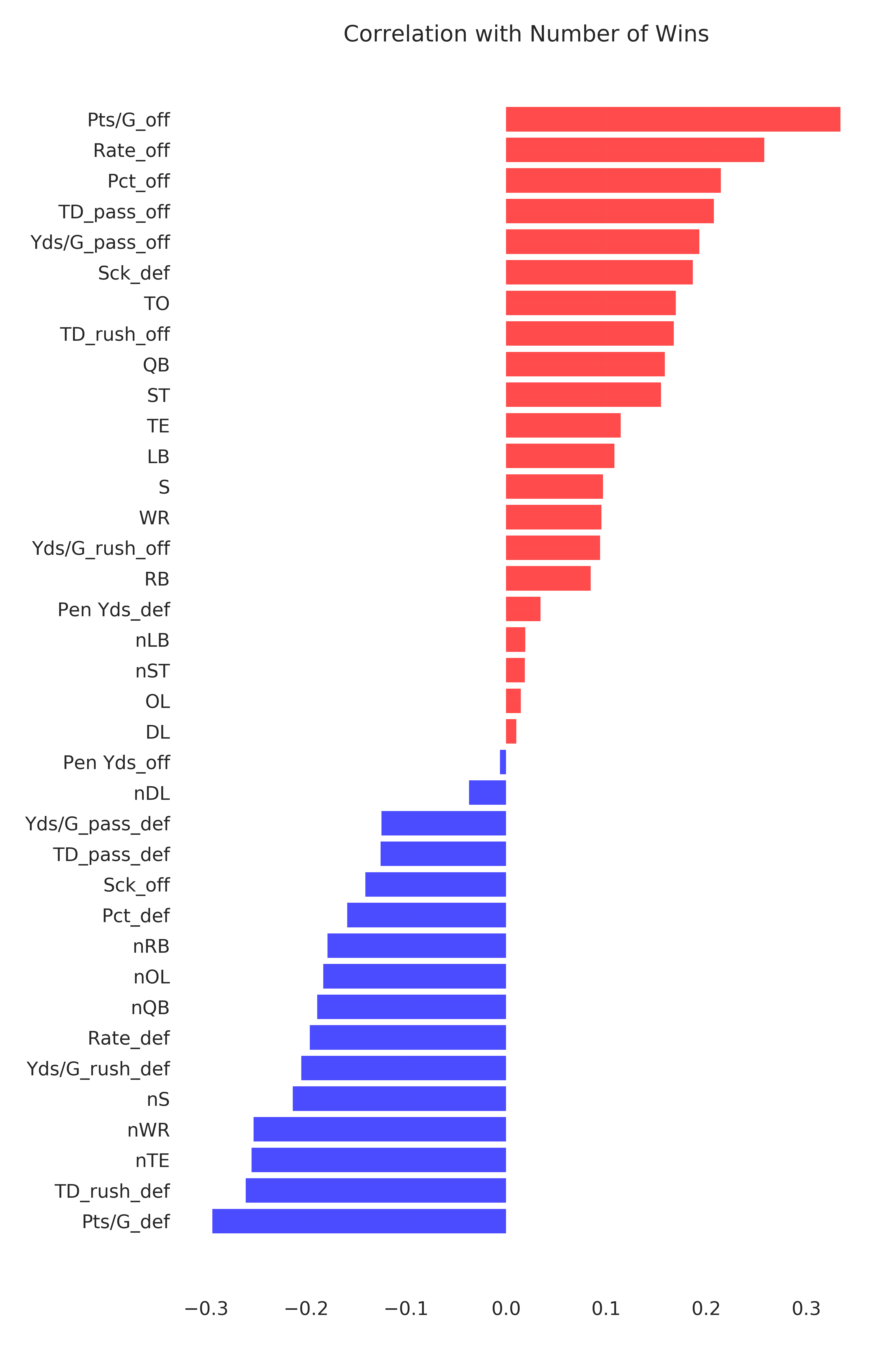
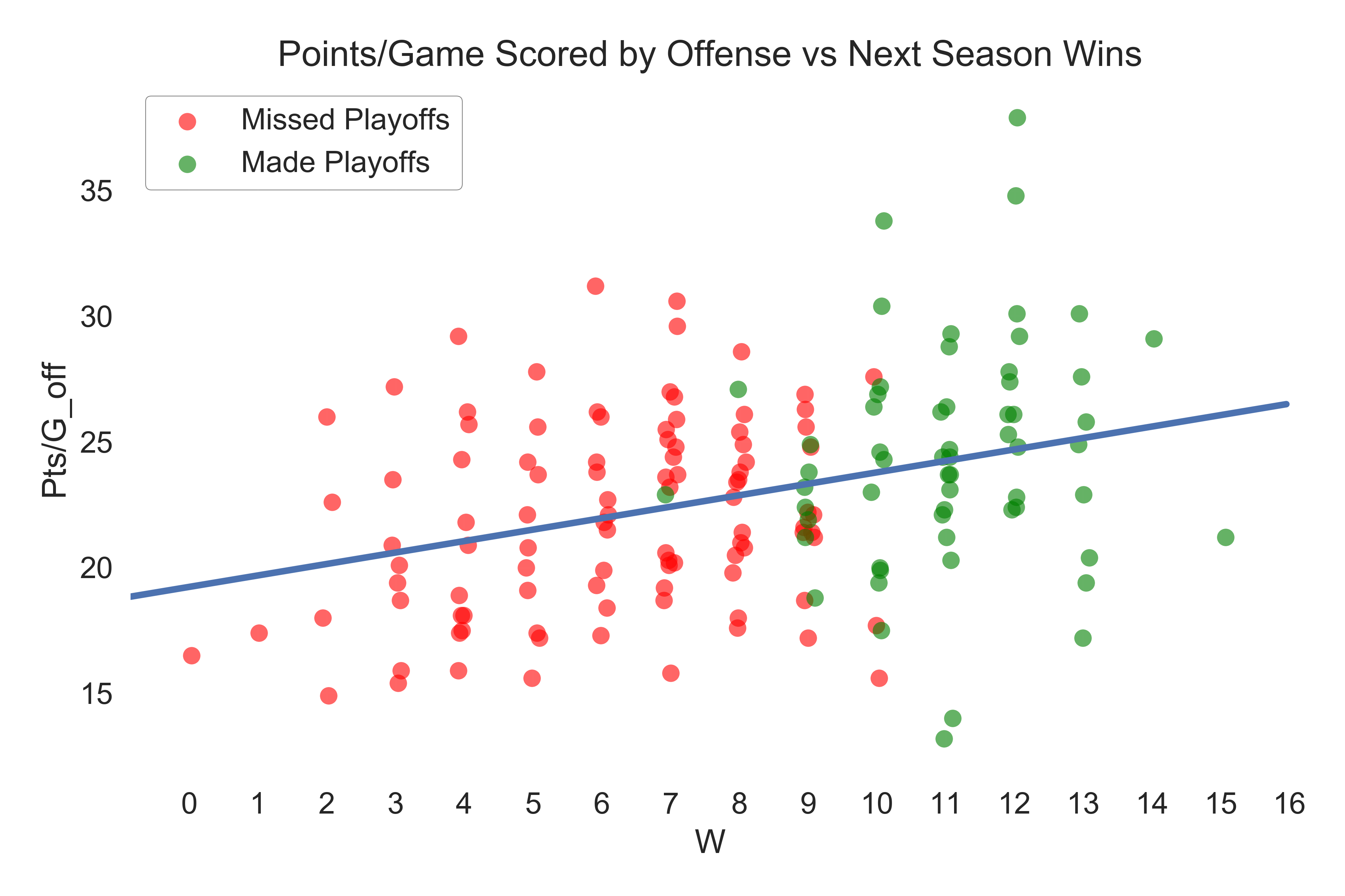
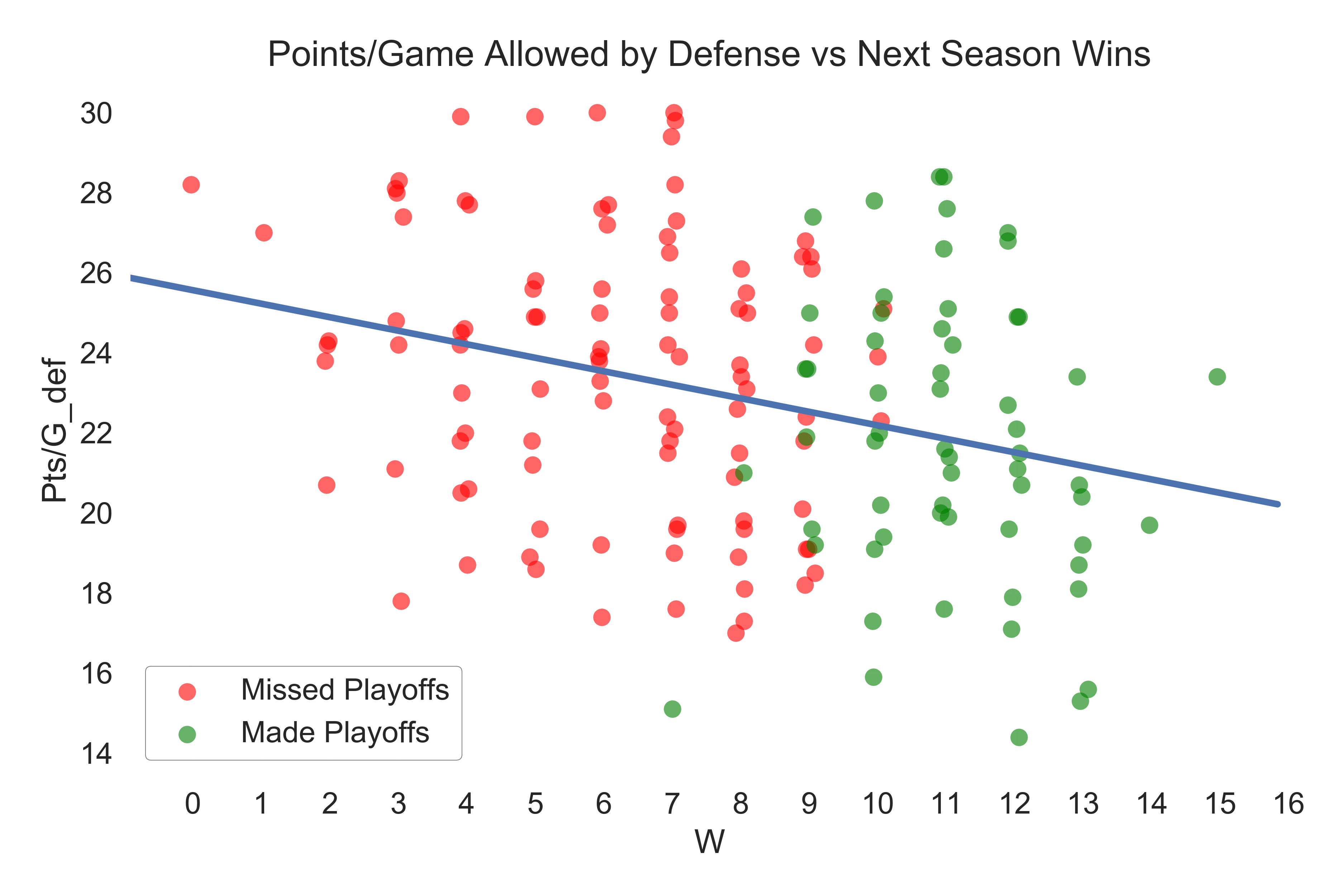
Points scored per game by the offense has the strongest positive correlation with wins and points allowed per game by the defense has the strongest negative correlation. These plots are shown below (I put a little jitter in the horizontal direction since wins is a discrete variable).

Also not alarming, as I mentioned earlier there is high inertia of professional sports. Something interesting that I noticed is that the number of tight ends, wide receivers, and secondary players on a team is negatively correlated with wins. Perhaps teams have an excess of these position players when there is not a big-time, reliable playmaker to rely on?

Modeling

For the modeling, I’ve decided that my target variable will be regular season win percentage. I’ll just divide the wins by 16 (the number of regular season games). I’m going to build several models and compare the results. I’ll also try blending some of the model results together in various ways.

2013-2016 will be my training set and 2017 will be my validation set. Ideally, I would like to have a train, test, and validation set, but since there is just a few seasons worth of data, this will have to do. I guess 2018 can be my test set…but that’s a long wait for the punchline.

I’ll use the coefficient of determination ($R^2$) and mean squared error ($MSE$) to evaluate initial model performance and compare models. Of more interest than these two quantities, however, is how the model does at predicting playoff teams once constrained by conference and division. What I mean is that after making predictions on win percentage,

I’ll separate the results by division (AFC East, NFC East, etc.). NFL playoffs consist of 12 teams: 8 division winners (4 from each conference) and 4 wild card teams (2 from each conference). The predicted winner of a division will be easy, it’s simply the highest predicted win percentage inside that division. Wild card teams are a bit trickier, but not much. After taking the 4 division winners in a conference, The 2 teams with the next 2 highest predicted win percentage will be the wild card teams. I’ll do this for both conferences until I have all 12 playoff teams that a specified model predicts.

As mentioned earlier, many of the features are highly correlated so I will need to employ some sort of feature selection into my modeling framework.

Forward Subset Selection Linear Regression with Leave One Out Cross Validation

I’ll start simple with a forward selection linear regression model. Forward selection is a feature selection technique which starts by fitting a series of one-variable models on all features. The features which yields the one-variable model with the best performance (MSE in this case), will be carried forward to the next round where a series of two-variable models are fitted with each of the remaining unused variables. The best two-variable model is then carried forward and so on until all features are in the model. I’ll keep track of MSE along the way to see which n-variable model yields the best validation performance.

There’s not a great package for subset selection in Python so I’ll do it the old fashioned way. I’ll be using leave one out cross validation, 10-fold would probably suffice and be much faster, but I’ve got time and wanted to see loocv in action. Here’s my implementation:

fs_models = {}

unused_vars = X.columns
model_vars = []

lr = LinearRegression()

loo = LeaveOneOut()

mse = []

for i in range(1, len(X.columns) + 1):
    best_mse = 1e100
    for var in unused_vars:
        loo_mse = []
        for train_index, test_index in loo.split(X):
            X_train, X_test = X.iloc[train_index], X.iloc[test_index]
            y_train, y_test = y.iloc[train_index][target_var], y.iloc[test_index][target_var]
            lr.fit(X_train[model_vars + [var]], y_train)
            y_pred = lr.predict(X_test[model_vars + [var]])
            loo_mse.append((y_test.values - y_pred) ** 2)
        if np.mean(loo_mse) < best_mse:
            best_mse = np.mean(loo_mse)
            best_var = var
    mse.append(best_mse)
    model_vars.append(best_var)
    unused_vars = unused_vars.drop(best_var)
    fs_models[i] = [best_mse, model_vars.copy()]

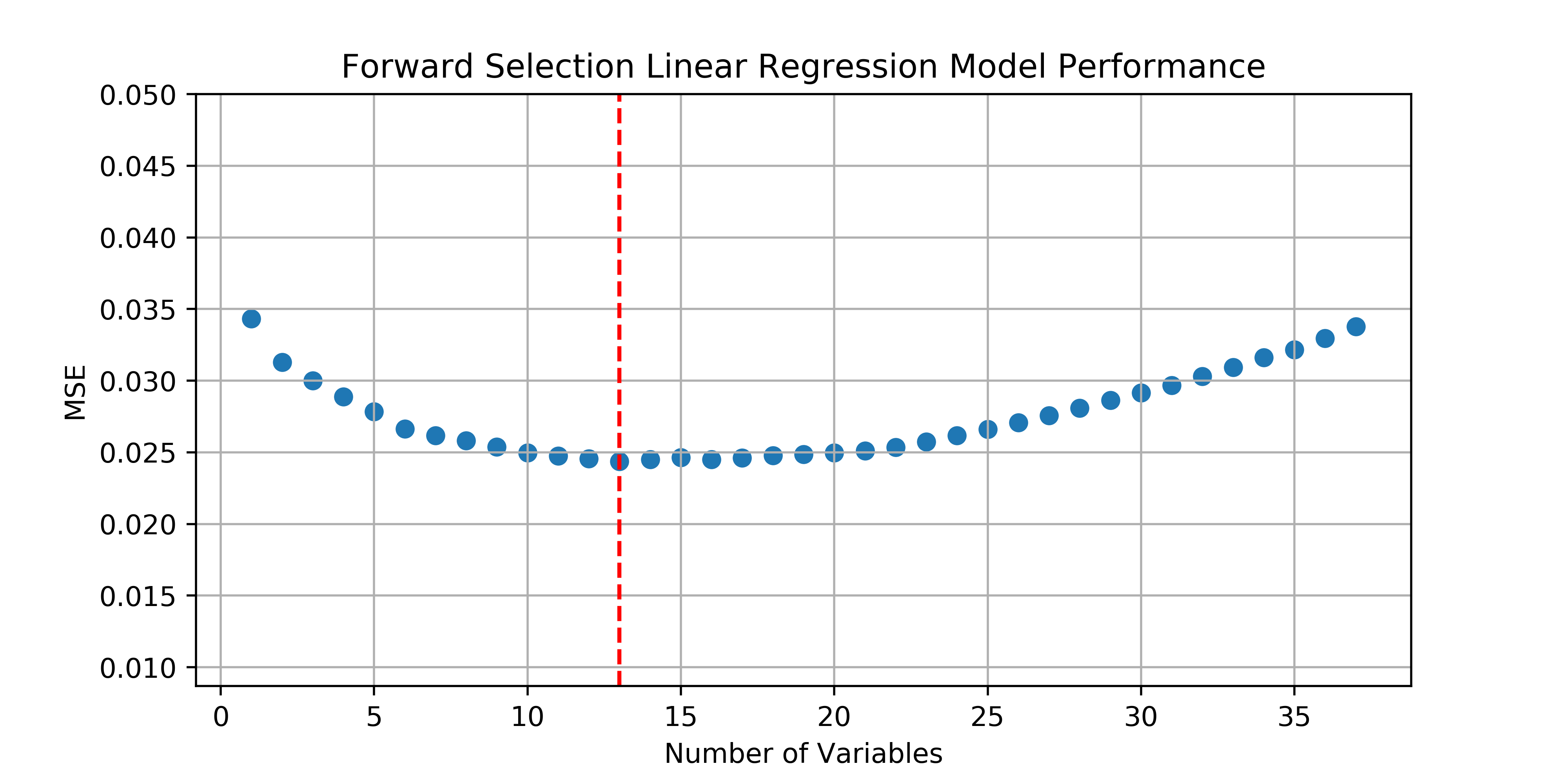
The best model contains 13 features and has a validation $R^2$ of 0.056…not great.

Linear Regression with Principal Component Analysis

For this next model, principal component analysis (PCA) will be my feature selection mechanism. I’ll iteratively fit models to an increasing number of principal components, keeping track of the 10-fold cross validation score along the way.

lr = LinearRegression()

cv_scores = []

for i in range(1, len(X.columns)+1):
    pca = PCA(n_components=i)
    X_pca = pca.fit_transform(X)
    lr.fit(X_pca, y[target_var])
    cv_scores.append(cross_val_score(lr, X_pca, y[target_var], cv=10).mean())

cv_scores = np.array(cv_scores)
best_n = cv_scores.argmax() + 1

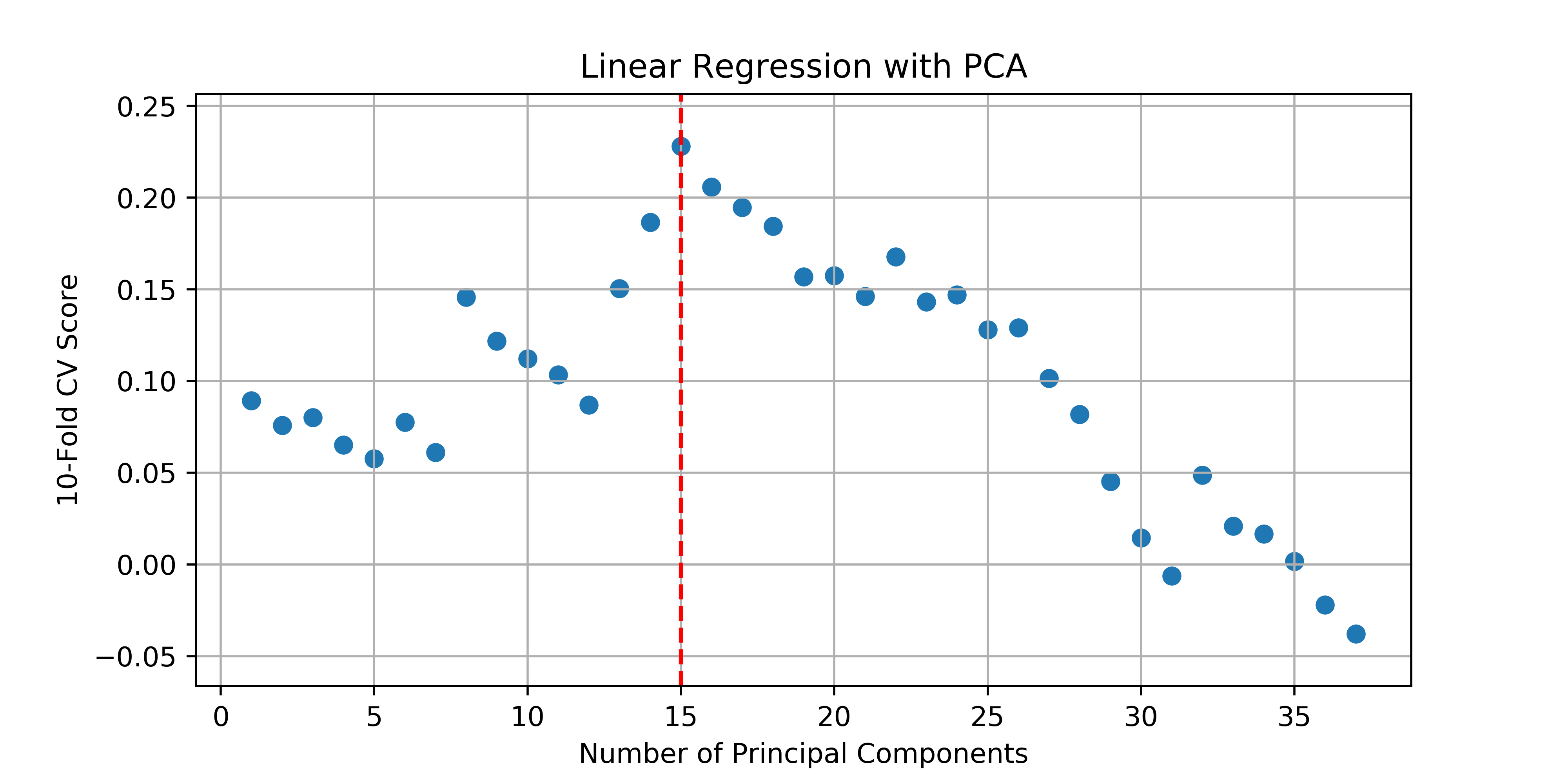
The best model that comes out of this uses the first 15 principal components as predictive features and has a validation $R^2$ of 0.138.

Lasso Regression

The Lasso regression algorithm inherently does feature selection by shrinking some of the linear regression coefficients to exactly zero via L1 regularization (unlike Ridge regression, which shrinks the regression coefficients toward but not to zero via L2 regularization). To tune the Lasso model, I’ll loop through an array of alpha values and choose the alpha value that results in the lowest 10-fold cross validation MSE.

alphas = np.linspace(.001, .1, 100)

lasso = Lasso()

kf = KFold(n_splits=10, random_state=rs)

mse = []
coefs = []
for a in alphas:
    lasso.set_params(alpha=a)
    kf_mse = []
    for train_index, test_index in kf.split(X):
        X_train, X_test = X.iloc[train_index], X.iloc[test_index]
        y_train, y_test = y.iloc[train_index][target_var], y.iloc[test_index][target_var]
        lasso.fit(X_train, y_train)
        y_pred = lasso.predict(X_test)
        kf_mse.append(np.mean((y_test.values - y_pred) ** 2))
    lasso.fit(X, y[target_var])
    coefs.append(lasso.coef_)
    mse.append(np.mean(kf_mse))
coefs = np.array(coefs)
mse = np.array(mse)

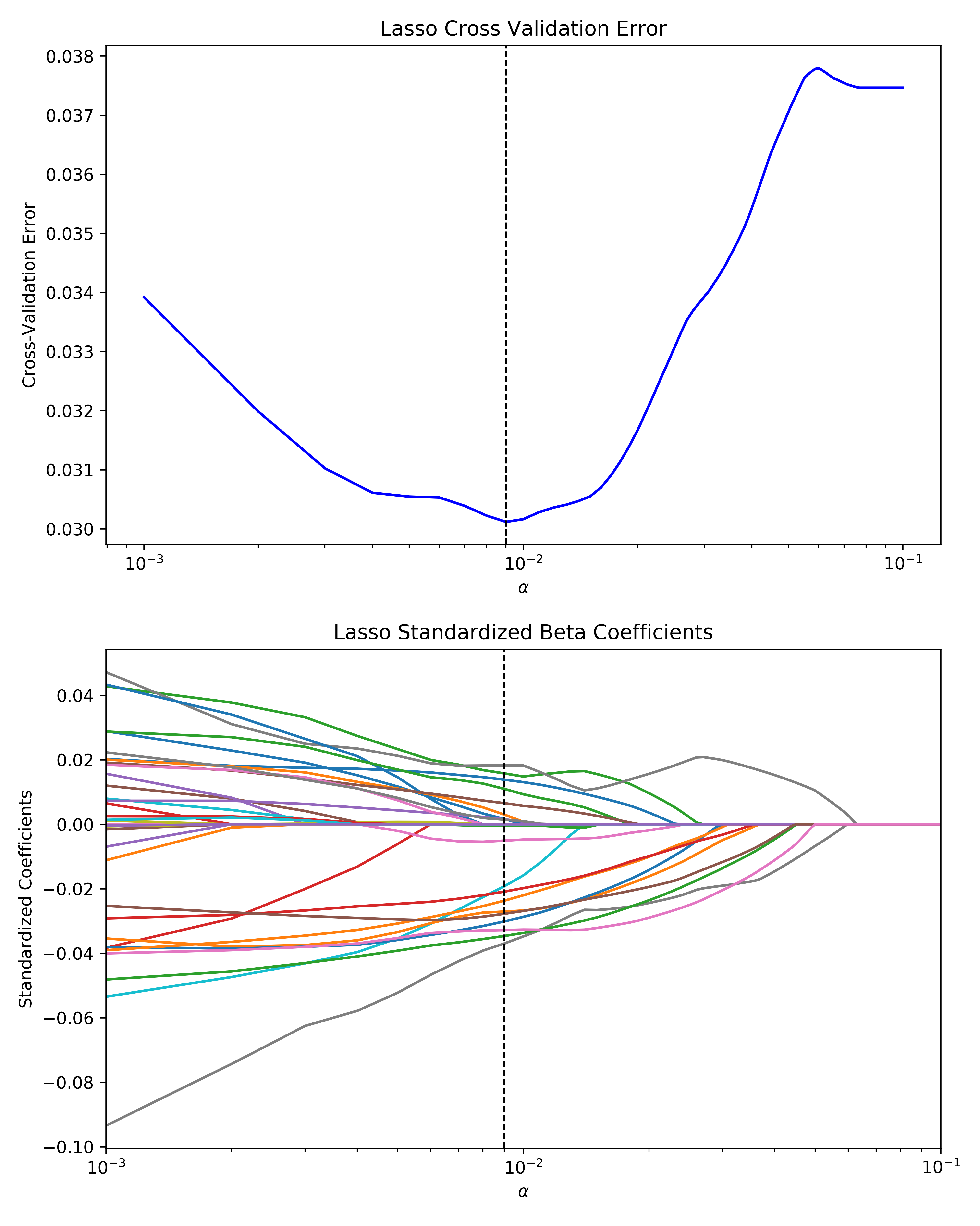
The best Lasso model that falls out of this has a validation $R^2$ of 0.225.

Random Forest with Grid Search

Last, I’ll create a random forest regression model using grid search to optimize some of the hyperparameters.

rf = RandomForestRegressor(n_estimators=100, random_state=rs)

param_grid = {
    'max_depth': range(1, 10),
    'min_samples_leaf': range(1, 4),
    'min_samples_split': range(2, 5)
}

gs = GridSearchCV(rf, param_grid, n_jobs=-1, cv=10)
gs.fit(X, y[target_var])

print(gs.best_params_)

{'max_depth': 4, 'min_samples_leaf': 1, 'min_samples_split': 2}

The random forest regression model with the above hyperparameters has a validation $R^2$ of 0.172. Here’s what the feature importance for this model looks like.

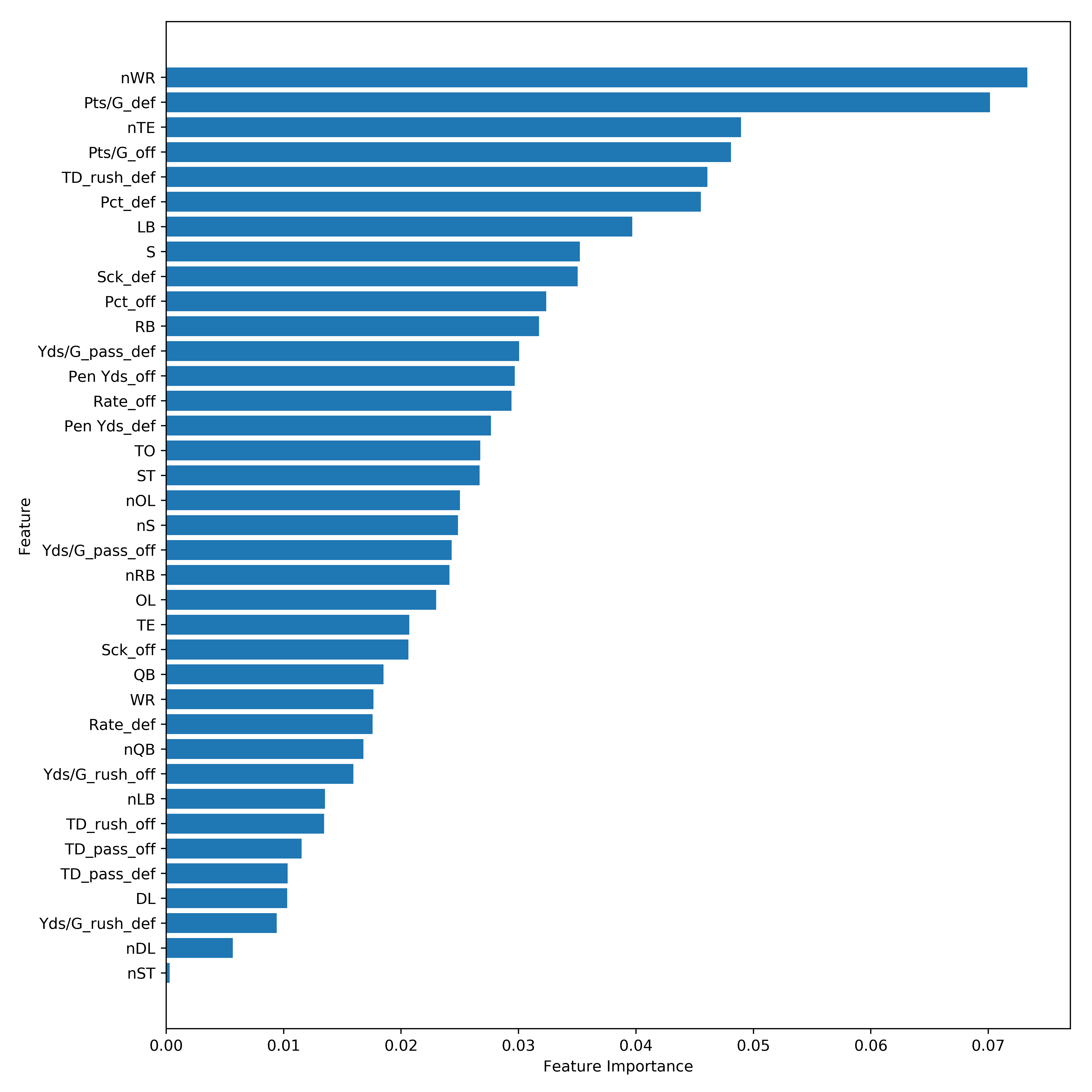
Well that’s unexpected…the number of wide receivers on a team is the most important feature in this model followed closely by points per game allowed by the defense in the previous season.

Blended Models

I tried 2 very simple blending techniques for this project. First was a simple average of the predictions of the 4 models described above which achieved a 0.209 validation $R^2$. The next was a linear regression of the 4 model predictions which achieved a validation $R^2$ of 0.286.

Results

After building, training, and making predictions, each of the 4 models and the 2 blended models were constrained by conference and division to get the final predictions for teams that would make the playoffs. Here’s what the actual playoff picture looked like in 2017:

AFC Division Winners: NE, PIT, JAC, KC
NFC Division Winners: PHI, MIN, NO, LA
AFC Wild Cards: BUF, TEN
NFC Wild Cards: CAR, ATL

Below is the result for each of the model. Green indicates a correctly predicted division winner or wild card team, orange indicates an incorrectly predicted division winner or wild card team but the team still made the playoffs in another capacity, while red indicates an incorrect prediction of a team that did not make the playoffs.

Forward Subset Selection Linear Regression

AFC Division Winners: NE, PIT, TEN, KC
NFC Division Winners: DAL, CHI, ATL, LA
AFC Wild Cards: JAC, DEN
NFC Wild Cards: PHI, DET

Division Winners: 3/8
Playoff Teams: 8/12

Linear Regression with Principal Component Analysis

AFC Division Winners: NE, PIT, TEN, OAK
NFC Division Winners: DAL, GB, ATL, LA
AFC Wild Cards: KC, DEN
NFC Wild Cards: PHI, MIN

Division Winners: 4/8
Playoff Teams: 8/12

Lasso Regression

AFC Division Winners: NE, PIT, TEN, KC
NFC Division Winners: DAL, MIN, ATL, LA
AFC Wild Cards: OAK, DEN
NFC Wild Cards: PHI, GB

Division Winners: 5/8
Playoff Teams: 8/12

Random Forest Regression

AFC Division Winners: NE, PIT, TEN, KC
NFC Division Winners: PHI, GB, ATL, SEA
AFC Wild Cards: OAK, BAL
NFC Wild Cards: MIN, DAL

Division Winners: 4/8
Playoff Teams: 7/12

Average of Predictions

AFC Division Winners: NE, PIT, TEN, KC
NFC Division Winners: DAL, GB, ATL, LA
AFC Wild Cards: OAK, DEN
NFC Wild Cards: PHI, MIN

Division Winners: 4/8
Playoff Teams: 8/12

Linear Regression of Predictions

AFC Division Winners: NE, PIT, TEN, KC
NFC Division Winners: DAL, MIN, ATL, SEA
AFC Wild Cards: OAK, BAL
NFC Wild Cards: PHI, GB

Division Winners: 4/8
Playoff Teams: 7/12

Discussion

Although the linear regression blended model had the highest coefficient of determination ($R^2$), the lasso regression model had the best performance once constrained by conference and division, correctly predicting 5/8 division winners and 8/12 playoff teams.

NFL Future Odds

Disclaimer: This project is purely for educational purposes and should not be used for placing any bets.

Every year at the beginning of the season, Vegas puts out odds for each team to win their respective division. The table below summarizes how I would have done if I had used this model to place a $100 bet on each of the predicted division winners prior to the 2017 NFL season.

Team	Odds	Bet	Winnings
New England Patriots	1:14	$100.00	$7.14
Pittsburgh Steelers	2:3	$100.00	$66.67
Tennessee Titans	2:1	$100.00	$0.00
Kansas City Chiefs	2:1	$100.00	$200.00
Dallas Cowboys	5:4	$100.00	$0.00
Minnesota Vikings	7:2	$100.00	$350.00
Atlanta Falcons	8:5	$100.00	$0.00
Los Angeles Rams	25:1	$100.00	$2,500.00
Total	-	$800.00	+$3,123.81

That’s a 390.48% return on investment. Clearly, picking the Los Angeles Rams to win their division at the beginning of last season would have been considered a long-shot but would have given solid winnings of \$2,500 on a \$100 bet. Even if that division were predicted incorrectly, I would have still achieved a 77.8% ROI. Not too shabby.

2018 Predictions

Here’s what the lasso regression model predicts for the 2018 season (and their current odds to win their division):

AFC Division Winners: NE(2:11), PIT(4:11), JAC(2:1), LAC(7:4)
NFC Division Winners: DAL(7:2), MIN(7:5), ATL(2:1), SEA(4:1)
AFC Wild Cards: BAL(9:2), TEN(7:2)
NFC Wild Cards: PHI(5:8), LA(4:5)

So there’s no long-shot odds for any of my predicted division winners, but if I placed \$100 bets on each of the 8 predicted division winners today (5/11/18), I stand to gain a profit \$1,519.54 if every prediction is correct.

Conclusion

So for this project I scraped positional spending, number of positional players, offensive statistics, defensive statistics, and standings from the web. After exploring the relationships between the independent and dependent variables, I built 4 models to make predictions with and tried 2 model blending techniques. The predictions were constrained by NFL conference and division to predict division winners and playoff teams by predicted win percentage. I then calculated what my return on investment would be had I used these predictions to make bets on division winners prior to the 2017 season. I also presented my future predictions and potential profits if bets were placed today. I’ll reiterate the disclaimer here just to CMA.

Disclaimer: This project is purely for educational purposes and should not be used for placing any bets.

Taylor Sansom

Coastal Hydrologist | Data Scientist

Predicting NFL Playoffs

Using positional salary spending and previous year stats to predict NFL playoff teams

Introduction

Getting the Data

Feature Descriptions

Exploratory Data Analysis

Modeling

Forward Subset Selection Linear Regression with Leave One Out Cross Validation

Linear Regression with Principal Component Analysis

Lasso Regression

Random Forest with Grid Search

Blended Models

Results

Forward Subset Selection Linear Regression

Linear Regression with Principal Component Analysis

Lasso Regression

Random Forest Regression

Average of Predictions

Linear Regression of Predictions

Discussion

NFL Future Odds

2018 Predictions

Conclusion