Model-Level Hydrodynamic Particle Tracking

All code for this project is located in the project repository HERE

Introduction

To support oyster reef restoration efforts and other potential projects (like oil spill response), I developed model-level particle tracking functionality for TxBLEND, a two-dimensional hydrodynamic and salinity transport model used by the Texas Water Development Board (TWDB) to simulate water circulation and salinity patterns in Texas estuaries. TxBLEND is a vertically-averaged, finite-element model which employs and unstructured, triangular element grid with linear basis functions. The model is designed specifically for Texas estuaries, which are generally very shallow and wide bodies of water.

Particle tracking studies are often conducted using velocity from model outputs, which typically have time scales of 30 minutes to one hour. The novelty of implementing particle tracking at the model-level is that the calculation of velocity, and subsequently position, happen on the model time-step. The typical time-step for TxBLEND model runs is two or three minutes. This allows me to capture smaller perturbations of the velocity field that would otherwise be lost to averaging when using hourly model output for example.

Interpolating Velocity in a Triangular Element

Figure 1 shows the representation of a linear triangular element, $l$, as it would appear in the TxBLEND model gird. The points $i$, $j$, and $k$ represent the nodes of the element $l$. All variable calculations (i.e. velocity, salinity, water level, etc.) occur at the nodes, and as a result, variable interpolations inside the element are straight-forward.

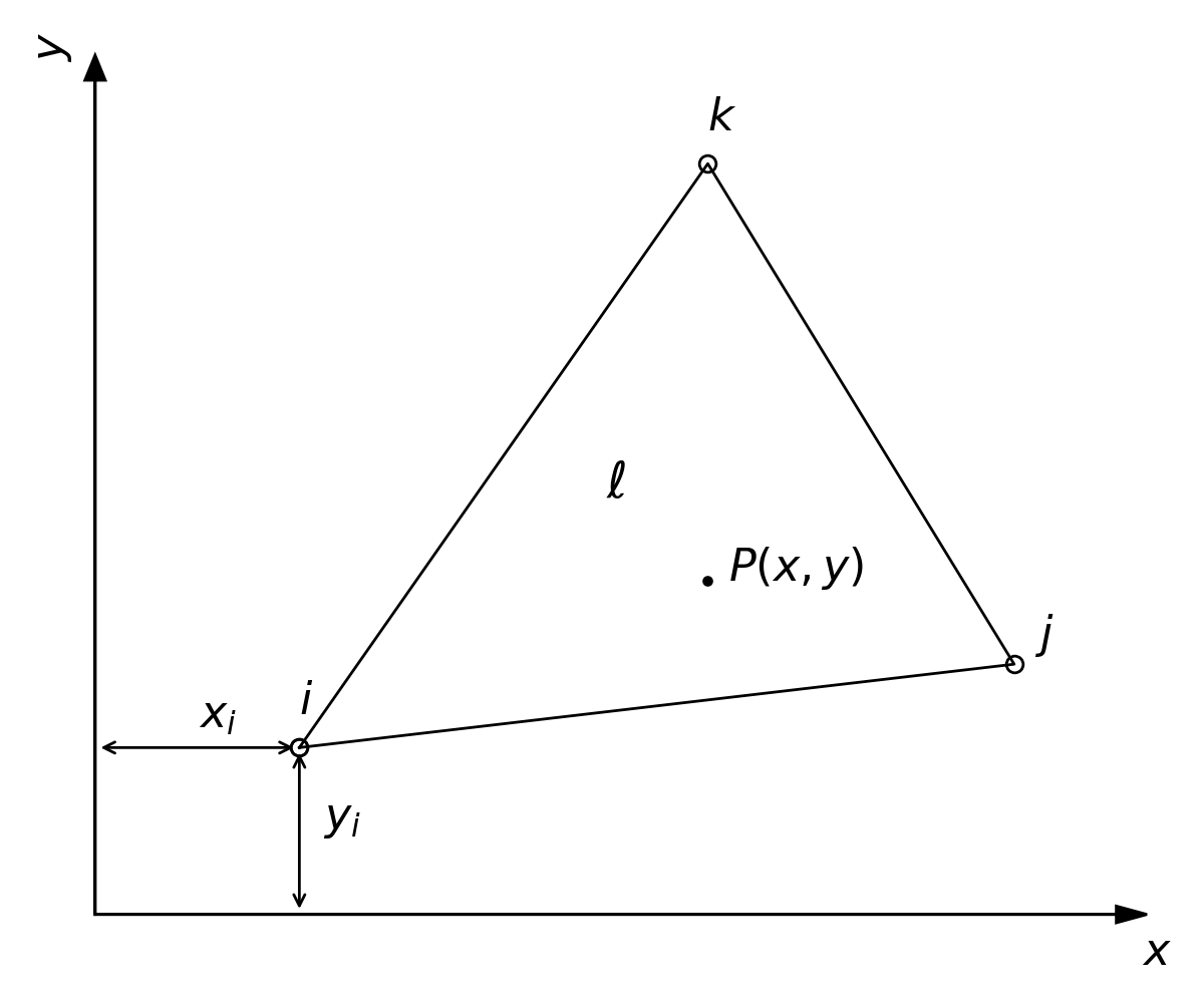
Figure 1. Schematic of a TxBLEND Element $l$.

To interpolate the velocity at point $P$ inside of a linear triangular element (see Figure 1), basis functions must first be calculated for each of the three nodes, or vertices, of the triangular with respect to the point $P$. The basis functions described herein are used as weighting functions and must fulfill the requirement that they are unity, or one, at the node for which they are calculated and zero at all other nodes. Also, in the case of linear triangles, they must describe a plane over the triangular element. The general expression for the $i$th basis function takes the form

$\phi_i = a_i + b_ix + c_iy$

where $a_i$, $b_i$, and $c_i$ are constants identified with the $i$th basis function, while $x$ and $y$ are the horizontal coordinates (i.e. longitude and latitude) of the point $P$. With this information, the $i$th basis function, $\phi_i$, can be written as

$\left \{ \begin{array} {1} \phi_i(x_i, y_i)\\ \phi_j(x_j, y_j)\\ \phi_k(x_k, y_k) \end{array} \right \} = \left \{ \begin{array} {1} 1\\0\\0 \end{array} \right \} = \begin{bmatrix} 1&x_i&y_i\\ 1&x_j&y_j\\ 1&x_k&y_k\\ \end{bmatrix} \begin{pmatrix} a_i\\b_i\\c_i \end{pmatrix}$

where $i$, $j$, and $k$ refer to the element nodes using counterclockwise convention, and the 3$\times$3 matrix is referred to as $\left [C\right ]$. Solvering for $a_i$, $b_i$, and $c_i$, we obtain

$\begin{align} \begin{split} a_i &= (x_jy_k-x_ky_j)/2A\\ b_i &= (y_j-y_k)/2A\\ c_i &= (x_k-x_j)/2A \end{split} \end{align}$

where $2A = \left [C\right ]$ is twice the area of the triangular element. Substituting equation $(3)$ into $(1)$, the basis function for node $i$ becomes

$\phi_i=\frac{(x_jy_k-x_ky_j)+(y_j-y_k)x+(x_k-x_j)y}{2A}.$

Analogous expressions for the basis functions for nodes $j$ and $k$ are easily obtained by cyclically permutating the indices $i$, $j$, and $k$ in $(4)$. The resulting expressions are

$\phi_i=\frac{(x_ky_i-x_iy_k)+(y_k-y_i)x+(x_i-x_k)y}{2A}$

and

$\phi_k=\frac{(x_iy_j-x_jy_i)+(y_i-y_j)x+(x_j-x_i)y}{2A}.$

Another property of basis functions that is satisfied by $(4)$, $(5)$, and $(6)$ is

$\phi_i+\phi_j+\phi_k=1$

which shows that the functions are not independent of each other, since given any two basis functions, the third is automatically specified by $(7)$.

Because velocity is calculated at each node, the interpolated velocity components at point $P$ are simply

$\begin{align} \begin{split} u_p &= \phi_iu_i+\phi_ju_j+\phi_ku_k\\ v_p &= \phi_iv_i+\phi_jv_j+\phi_kv_k \end{split} \end{align}$

where $u_p$ and $v_p$ are the velocity components in the $x$-direction (East-West) and $y$-direction (North-South) at point $P$ respectively.

Calculating Particle Position

Initial positions of the particles are specified prior to running the TxBLEND model, which I’ll discuss in the application section. Subsequent particle positions for the remainder of the model run must be calculated at each model time-step based on interpolated velocity as discussed in the previous section. This implementation of particle tracking uses a two-level, time-averaged velocity for better accuracy in calculating the particle movement. Additionally, to simulate the spreading of particles due to dispersion and spat movement (in the context of oyster larvae), a random walk component is added to the velocity vector.

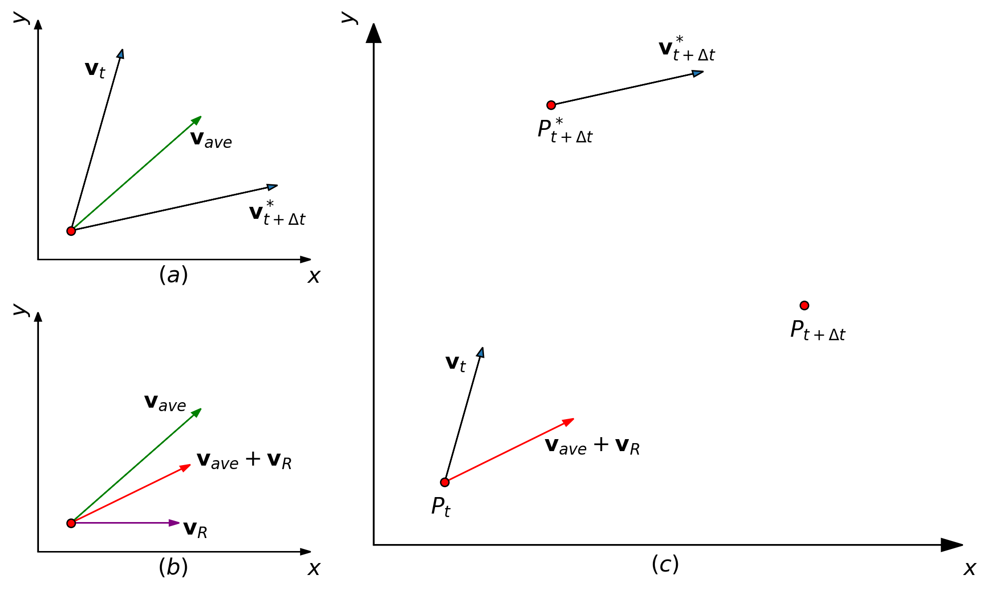
Figure 2. Schematic of particle position calculations.

Consider a single particle with an initial position of $P_t$ and corresponding interpolated velocity components $u_t$ and $v_t$. The subscript $t$ denotes the value of each variable at the current model iteration, or time-step, while a subscript $t+\Delta t$ indicates the value of each variable at the next model iteration. For simplicity, the velocity components $u$ and $v$ will be represented in vector notation $\mathbf{v}$. The variable $\Delta t$ is the model time-step and is typically two or three minutes for TxBLEND. To calculate the particle’s position at the next time-step, $P_(t+\Delta t)$, a temporary position is first calculated with

$P_{t+\Delta t}^* = P_t + v_t\Delta t$

where $v_t$ is the velocity at time $t$ (see Figure 2(c)). Next, a temporary interpolated velocity, $v_{t+\Delta t}^*$, is calculated at the temporary position, $P_{t+\Delta t}^*$, using the methods described earlier. The calculated velocities at the two time-steps are then averaged with

$v_{ave}=\frac{v_t+v_{t+\Delta t}^*}{2},$

which is used to move the particle from its initial position, $P_t$, to its position at the next time-step, $P_{t+\Delta t}$ (see Figure 2(a)).

As mentioned earlier, a random walk velocity component is also added to simulate the spreading of particles due to dispersion. This random walk is obtained by constructing a velocity range which is proportional to a typical value for the dispersion coefficient, and multiplying it by a random number, $R$, which is generated from a continuous, uniform distribution on the interval -0.5 and 0.5. The velocity range is given by

$v_{range} = \sqrt{6\frac{D}{\Delta t}}$

where $D$ is the dispersion coefficient and is typically equal to 100 $\frac{ft^2}{s}$. The random walk velocity then becomes

$v_R=v_{range}*R$

and can be seen in Figure 2(b). With this information, the particle’s position at time $t+\Delta t$ can be calculated by

$P_{t+\Delta t}=P_t+(v_{ave}+v_R)*\Delta t.$

Applying Particle Tracking to an Estuary System

The techniques discussed thus far have considered only a single particle, but can be scaled up to accommodate any reasonable number of particles. For the following case studies, a total of 1,000 particles were released over the course of the first 20 hours of model runtime in 10 batches of 100 particles. To simplify initial velocity calculations in the model, the initial positions of the particles are limited to being located along element edges, or node strings (see Figure 3). Additionally, all 10 particle releases use these 100 initial particle positions as a starting point. After the initial release, each particle position is updated at every model iteration.

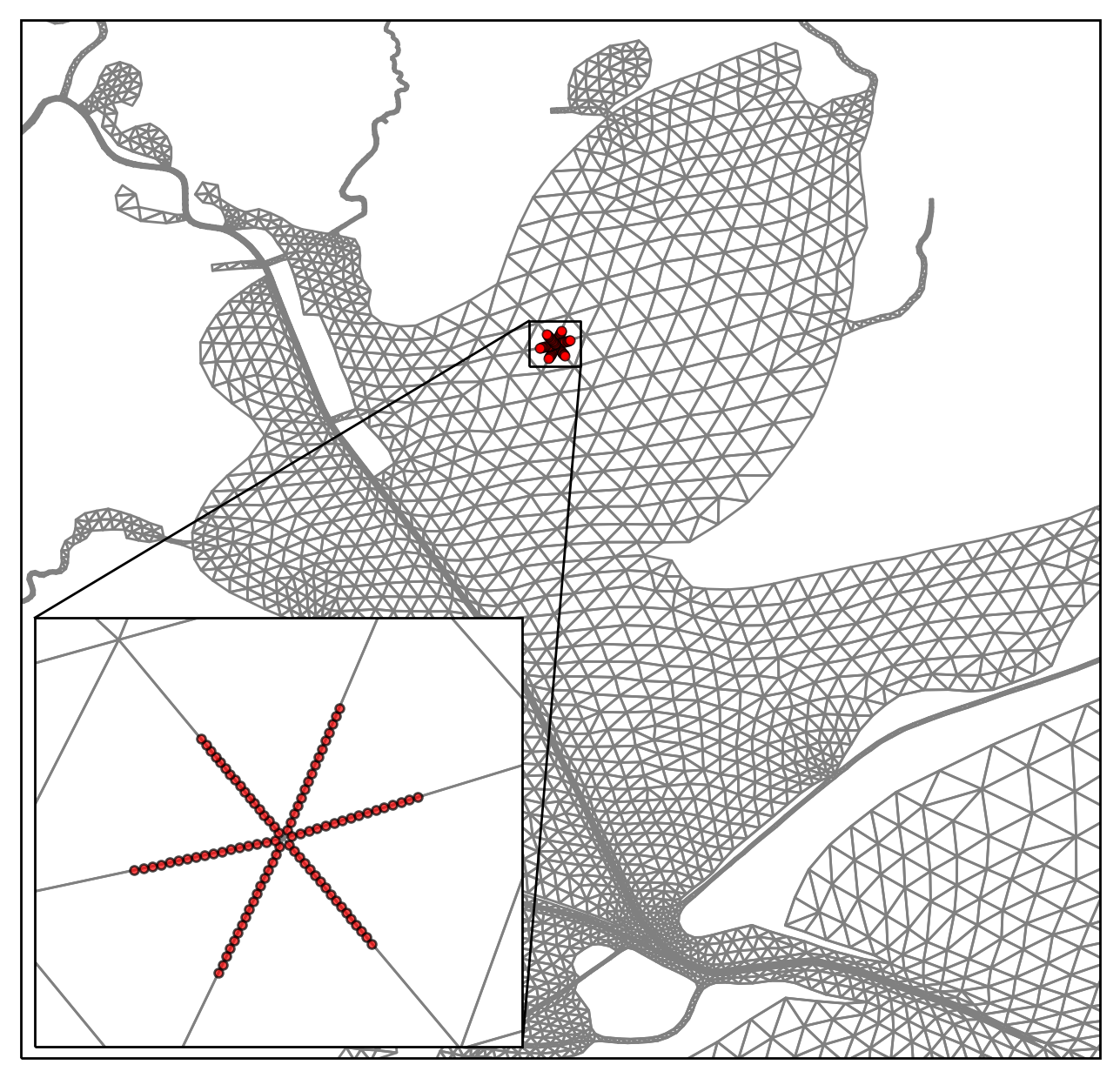
Figure 3. Initial particle locations for a potential sanctuary reef in upper Trinity Bay.

Although particle position is tracked on a two or three minute time interval, the model output for particle position is bihourly. The reasoning for this is that the spatiotemporal domain of the model is much larger than both the model time-step and the change in position of a particular particle between model time-steps. Increasing the frequency of model output adds little value to the inferences that can be made from the particle tracking simulation and would add an unnecessary burden on my finite storage limitations.

In addition to tracking particles on a bihourly basis, I also include hourly velocity vectors at several carefully chosen nodes and daily average salinity over the entire model domain. The velocity vectors help to mentally grasp why the particles move in the way they do, which is especially helpful in deep-draft ship channels, entrance channels, and riverine inflow points. Also, because oyster larvae viability can be dependent on the salt content of a water column, the salinity contours aid in roughly estimating the survival rate of oyster larvae, although this is beyond the scope of this report.